Neurokognition II

SS2019

Prüfungstermine

Die Prüfungen zur Neurokognition finden zu folgenden Terminen statt:
1. August, 12. August, 23. September 2019,

Anmeldungen bitte direkt an Frau Susan Köhler, susan.koehler@informatik.tu-chemnitz.de.

Inhalte

Die Veranstaltung führt in die Modellierung neurokognitiver Vorgänge des Gehirns ein. Neurokognition ist ein Forschungsfeld, welches an der Schnittstelle zwischen Psychologie, Neurowissenschaft, Informatik und Physik angesiedelt ist. Es dient zum Verständnis des Gehirns auf der einen Seite und der Entwicklung intelligenter adaptiver Systeme auf der anderen Seite. Die Neurokognition II beleuchtet komplexere Modelle von Neuro-psychologischen Prozessen, mit dem Ziel neue Algorithmen für intelligente, kognitive Roboter zu entwickeln. Themen sind Wahrnehmung, Gedächtnis, Handlungskontrolle, Emotionen, Entscheidungen und Raumwahrnehmung. Zum tieferen Verständnis erfordern die Übungen auch praktische Aufgaben am Rechner.

Randbedingungen

Empfohlene Voraussetzungen: Grundkenntnisse Mathematik I bis IV, Neurokognition I

Prüfung: Mündliche Prüfung

Ziele: Fachspezifische Kenntnisse der Neurokognition

Syllabus

Part I Introduction

The introduction motivates the goals of the course and basic concepts of models. It further explains why computational models are useful to understand the brain and why cognitive computational models can lead to a new approach in modeling truly intelligent agents.

The styles of computation used by biological systems are fundamentally different from those used by conventional computers: biological neural networks process information using energy-efficient asynchronous, event-driven, methods. They learn from their interactions with the environment, and can flexibly produce complex behaviors. These biological abilities yield a potentially attractive alternative to conventional computing strategies.

Neurokognition II is particularly devoted to model perception cognition and behavior in large-scale neural networks. The course introduces models of early vision, attention, object recognition, space perception, cognitive control, memory, emotion and consciousness.

Exercise I.1: Tutorial on the neuro-simulator ANNarchy, files: exerciseI.1.zip.

Part II Early Vision

Perhaps our most important sensory information about our environment is vision. The lecture "early vision" explains the first processing steps of visual perception.

Overview:
Adelson, E. H., Bergen, J R. (1985): Spatiotemporal energy models for the perception of motion. J. Opt. Soc. Am. A. 2:284-299
DeAngelis, G., Ohzawa, I., Freeman, R.D. (1995): Receptive-field dynamics in the central visual pathways. TINS Vol. 18, No. 10, 1995

2.1 The Retina and LGN

Vision starts in the retina, which is considered part of the brain. The lecture explains the concept of a receptive field and introduces simple models of early processing that model dynamic receptive fields.

Additional Reading:
Cai D, DeAngelis GC, and Freeman RD (1997) Spatiotemporal receptive field organization in the LGN of cats and kittens. J Neurophysiol 78:1045-1061.

2.2 Shape perception

Shape perception refers to the fact that the visual system has filters that respond optimally to oriented bars or edges, which takes place in area V1, also called striate cortex. This lecture introduces into the receptive fields of neurons in V1 and explains what kind of information V1 encodes with respect to shape perception.

Exercise II.1: Gabor filters, Files: exerciseII.1.zip

2.3 Color

Color perception starts in the retina, since we have receptors that are selective for different wavelength of the light. This lecture introduces into models of color selective receptive fields.

2.4 Cortical magnification

In the cortex, the visual space is overrepresented in the fovea, which means that much more space in cortex is devoted to compute information around the center of visual space. A cortical magnification function allows to model the relation between visual and cortical space providing a method to account for the overrepresentation in models of visual perception.

2.5 Motion

Motion perception begins already in area V1 by motion sensitive cells and then continues in the dorsal pathway in areas MT and MST.

2.6 Depth

Seeing in three dimensions requires to extract depth information from the visual scene. One method, called binocular disparitiy, is of primary focus.

Exercise II.2: Depth perception, Files: exerciseII.2.zip, solution Part B

2.7 Gain Normalization

Gain normalization appears to be a canonical neural computation in sensory systems and possibly also in other neural systems. Gain normalization is introduced and examples for normalization in retina, in primary visual cortex, in higher visual cortical areas and in non-visual cortical areas are given.

2.8 Learning

Why does the brain develop a particular set of feature detectors for early vision. This lecture addresses how approaches that rely on learning allow to better understand the coding of vision in the brain.

Additional Reading:
Simoncelli, E.P., Olshausen, B. A.: Natural Image Statistics and Neural Representation. Annu. Rev. Neurosci. 2001. 24:1193-216
Simoncelli, E.P.: Vision and the statistics of the visual environment. Current Opinion in Neurobiology 2003, 13:144-149.

Part III High-level Vision

High-level vision deals with questions of how we recognize objects or scenes and how we direct processing resources to particular aspects of visual scenes (visual attention).

3.1 Object recognition

Object recognition appears to be solved by a hierarchically organized system that progressively increases the complexity and invariance of feature detectors.

Exercise III.1: Object Recognition and HMAX, Files: exerciseIII.1.zip ; article: Serre, Wolf and Poggio (2004).

3.2 High-Level Vision: Visual Attention

Attention refers to mechanisms that allow the focusing of processing resources. Experimental observations, neural principles and system-level models of attention are described.

Exercise III.2: Normalization model of attention, Files: exerciseIII.2.zip solution Part B.

Exercise III.3: Visual attention and experimental data, Files: exerciseIII.3.zip .

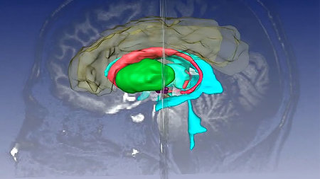
3.3 High-Level Vision: Space Perception

The perception of space is very crucial for systems that interact with the world. This lecture introduces to anatomical pathways of space perception. The primary focus is then directed to the problem of "Visual Stability", which deals with the question of why we perceive a stable environment regardless that each eye movement changes the content on the retina.

Additional Material:

Video: Setup for predictive remapping

Setup for predictive remapping (left: fixation task, right: saccade task) over time with respect to the three input signals (retinal signal (green), PC signal (red) and CD signal (blue)): A stimulus is shown either in the receptive field (RF; left) or in the future RF (FRF; right) while the eyes fixate the fixation point (FP). In the saccade task, an eye movement is executed to the saccade target (ST) afterwards. The green star depicts the current stimulus position, the red cross symbolizes the current eye position. As the retinal signal and the origin of the corollary discharge signal are retinotopic, they shift with the eye movement. In contrast, the PC signal is head-centered and therefore fixed during the saccade. The time in ms is aligned to saccade onset.

Video: Setup for spatial updating of attention with cued attention

Setup for spatial updating of attention with cued attention over time with respect to the three input signals (retinal signal (green), PC signal (red) and CD signal (blue)): A stimulus is presented at the attention position (AP) while the eyes fixate the fixation point (FP). Afterwards, an eye movement is executed to the saccade target (ST). The green star depicts the current stimulus position, the red cross symbolizes the current eye position. Place markers for the remapped and the lingering attention position (RAP and LAP) are shown. As the retinal signal and the origin of the corollary discharge signal is retinotopic, it shifts with the eye movement. In contrast, the PC signal is head-centered and therefore fixed during the saccade. The time in ms is aligned to saccade onset.

Video: Setup for spatial updating of attention with top-down attention

Setup for spatial updating of attention with top-down attention over time with respect to the three input signals (PC signal (red), CD signal (blue) and attention signal (orange)): An eye movement is executed from the fixation point (FP) to the saccade target (ST). During the whole process, top-down attention is introduced at the attention position (AP). The red cross symbolizes the current eye position. Place markers for the remapped and the lingering attention position (RAP and LAP) are shown. The corollary discharge signal is retinotopic, thus, it shifts with the eye movement. In contrast, PC signal and attention signal are head-centered and therefore fixed during the saccade. The time in ms is aligned to saccade onset.

Video: Simulation results of the two predictive remapping tasks

Simulation results of the two predictive remapping tasks (fixation and saccade task) over time. The activity of both LIP maps projected onto two two-dimensional planes representing horizontal and vertical information as well as the setup including the neural activities of both LIP maps projected into the retinotopic space are plotted. In the fixation task, the projected activity of LIP PC and LIP CD results in activity at RF (red and blue blob). In the saccade task, the projected activity of LIP PC and LIP CD results in activity at FRF (red and blue blob). Shortly before saccade onset, LIP CD triggers an additional activity blob at RF (blue blob). Both activity blobs are encoded in a retinotopic reference frame, thus, they move according to the eye movement. The time in ms is aligned to saccade onset.

Video: Simulation results of spatial updating of attention with cued attention

Simulation results of spatial updating of attention with cued attention over time. The activity of both LIP maps projected onto two two-dimensional planes representing horizontal and vertical information as well as the setup including the neural activities of both LIP maps projected into the retinotopic space are plotted. At the beginning, the activity in LIP PC and LIP CD triggers an attention pointer at AP (red and blue blob). Shortly before saccade onset, there is a second attention pointer triggered at RAP by LIP CD (blue blob). Both attention pointers are shifted with the eye movement as they are retinotopic. After the saccade, the CD signal decays and with it the activity in LIP CD as well as the second attention pointer. Furthermore, the PC signal updates to the correct postsaccadic eye position and thus, the attention pointer triggered by LIP PC updates to the correct position (AP). The time in ms is aligned to saccade onset.

Video: Simulation results of spatial updating of attention with top-down attention

Simulation results of spatial updating of attention with top-down attention over time. The activity of both LIP maps projected onto two two-dimensional planes representing horizontal and vertical information as well as the setup including the neural activities of both LIP maps projected into the retinotopic space are plotted. At the beginning, the activity in LIP PC triggers an attention pointer at AP (red blob). Shortly before saccade onset, there is a second attention pointer triggered at RAP by LIP CD (blue blob). Both attention pointers are shifted with the eye movement as they are retinotopic. After the saccade, the CD signal decays and with it the activity in LIP CD as well as the second attention pointer. Furthermore, the PC signal updates to the correct postsaccadic eye position and thus, the attention pointer triggered by LIP PC updates to the correct position (AP). The time in ms is aligned to saccade onset.