Computer Algebra with SymPy - Mathematical Programming

In this section, we introduce the Python module SymPy, which allows us to perform symbolic computations. In particular, we will learn how to:

work with mathematical expressions,
differentiate and integrate functions,
solve (nonlinear) systems of equations,
and handle simple differential equations.

First, we need to install the package, for example via our conda environment:

conda install -c conda-forge sympy

Then we import the module into our Python script:

import sympy as sy

Working with Functions¶

Let us begin by defining a mathematical function. To do this, we first need to declare a symbolic variable and then specify the functional expression:

x = sy.symbols('x')
f = x**3/3 - 2*x**2 + 3

The variable x is of type

type(x)

sympy.core.symbol.Symbol

and the expression f is of type

type(f)

sympy.core.add.Add

Objects of type sympy.core.add.Add are created by the addition of multiple expressions. The individual terms can be accessed via the attribute args:

f.args

(3, -2*x**2, x**3/3)

The three arguments themselves are again symbolic expressions that result from further arithmetic operations:

g1 = f.args[0]
print("First term", g1, "of type", type(g1))

g2 = f.args[1]
print("Second term", g2, "of type", type(g2))

g3 = f.args[2]
print("Third term", g3, "of type", type(g3))

First term 3 of type <class 'sympy.core.numbers.Integer'>
Second term -2*x**2 of type <class 'sympy.core.mul.Mul'>
Third term x**3/3 of type <class 'sympy.core.mul.Mul'>

The expression g1 is simply the number 3.0, while g2 and g3 are of type sympy.core.mul.Mul. These arise from the multiplication of symbolic expressions.

A mathematical expression is internally represented as a tree structure (expression tree). We can display the full internal representation using the following command:

sy.srepr(f)

"Add(Mul(Rational(1, 3), Pow(Symbol('x'), Integer(3))), Mul(Integer(-1), Integer(2), Pow(Symbol('x'), Integer(2))), Integer(3))"

Perhaps this examination has already given us a rough idea of how symbolic expressions are structured internally. However, we will not go into the exact details here.

Now let us take a look at what we can do with the function we have just defined.

Evaluating Symbolic Expressions¶

Symbolic expressions can also be evaluated for specific values of the variables. For this, we use the method subs (substitute), which allows us to replace a symbolic variable with a numerical value.

f.subs(x, 2)

Here, the variable x in the expression f is replaced by the value 2, and the result is computed.

We can also replace multiple variables at the same time. To do this, we pass a dictionary with the desired substitutions:

x, y = sy.symbols("x y")
g = x**2 + y**2

r = g.subs({x:1, y:2})

print(f"r = {r} ({type(r)})")

r = 5 (<class 'sympy.core.numbers.Integer'>)

The result of this operation is still a symbolic expression. If we want a numerical evaluation as a floating-point number, we can additionally use the method evalf():

r.evalf()

Simplifying Expressions¶

SymPy can also simplify and transform mathematical expressions. This is especially useful when symbolic computations lead to complicated intermediate results.

Let us first consider the following expression:

f = (x**2 - 1)/(x-1)

Mathematically, we know that

\frac{x^2-1}{x-1} = x+1

(1)

for all $x \ne 1$ . With the function simplify, SymPy can attempt to perform such simplifications automatically:

sy.simplify(f)

With expand, products can be expanded:

f = (x+1)**3
sy.expand(f)

The function factor, on the other hand, tries to factorize an expression:

f = x**2 - 1
sy.factor(f)

These functions are particularly useful when we want to further process symbolic computations or make mathematical structures more visible.

Differentiation¶

To compute the derivative of a symbolic expression with respect to a symbolic variable, we can either use the diff method, which is available for all SymPy expressions,

f = x**3/3 - 2*x**2 + 3
Df = f.diff(x)
print("Derivative:")
Df

Derivative:

or use the free function sympy.diff:

Df = sy.diff(f,x)
print("Derivative:")
Df

Derivative:

Both variants yield the same result.

Of course, SymPy can also differentiate more complex functions. Note that we must use the corresponding functions from the SymPy module for all mathematical functions:

g = sy.exp(-x**2)*sy.sin(x)
g.diff(x)

Higher-order derivatives and partial derivatives¶

With SymPy, higher-order derivatives of a symbolic expression can also be computed.
To do this, you can either call the .diff method multiple times or directly provide a second parameter specifying how many times to differentiate.

Example:

x = sy.symbols('x')

# First derivative
Df1 = f.diff(x)
print("First derivative:", Df1)

# Second derivative
Df2 = f.diff(x, 2)
print("Second derivative:", Df2)

# Third derivative
Df3 = f.diff(x, 3)
print("Third derivative:", Df3)

First derivative: x**2 - 4*x
Second derivative: 2*(x - 2)
Third derivative: 2

SymPy also allows us to symbolically differentiate functions with multiple variables. We can compute partial derivatives with respect to each variable, as well as mixed derivatives.

x, y = sy.symbols('x y')

# Define function
h = x**2 * y + sy.sin(x*y)

# Partial derivative with respect to x
df_dx = h.diff(x)
print("Partial derivative with respect to x:", df_dx)

# Partial derivative with respect to y
df_dy = h.diff(y)
print("Partial derivative with respect to y:", df_dy)

# Second derivative with respect to x
d2f_dx2 = h.diff(x, 2)
print("Second derivative with respect to x:", d2f_dx2)

# Mixed derivative: first x, then y
d2f_dxdy = h.diff(x).diff(y)
print("Mixed derivative d²f/(dx dy):", d2f_dxdy)

# Alternatively, you can specify both derivatives directly in one step
d2f_dxdy_alt = h.diff(x, y)
print("Mixed derivative (direct):", d2f_dxdy_alt)

Partial derivative with respect to x: 2*x*y + y*cos(x*y)
Partial derivative with respect to y: x**2 + x*cos(x*y)
Second derivative with respect to x: y*(-y*sin(x*y) + 2)
Mixed derivative d²f/(dx dy): -x*y*sin(x*y) + 2*x + cos(x*y)
Mixed derivative (direct): -x*y*sin(x*y) + 2*x + cos(x*y)

Integration¶

With the integrate method, we can compute the antiderivative (primitive) of a function:

F = f.integrate(x)
print("Antiderivative:")
F

Antiderivative:

Sometimes SymPy is overwhelmed by overly complex functions. In such cases, the integrate method simply returns the symbolic expression:

G = g.integrate(x)
print("Antiderivative:")
G

Antiderivative:

Definite integrals:

We can also compute definite integrals by passing a tuple consisting of the integration variable and the two bounds as the second parameter:

v = sy.integrate(f, (x, 0, 1))
print("Integral of f with bounds 0 and 1:")
v

Integral of f with bounds 0 and 1:

Improper integrals:

To compute improper integrals, for example $\int_0^\infty g(x)\,\mathrm dx$ , you simply use sy.oo (infinity) as the upper bound:

g = x**2*sy.exp(-x)
v = sy.integrate(g,(x,0,sy.oo))
print("Improper integral:")
v

Improper integral:

Power series¶

SymPy provides many useful functions for working with series, in particular sympy.series(...). With this function, we can compute the Taylor or power series of a function of any order:

G = g.series(x, 0, 4)  # Taylor approximation at expansion point 0, up to order 4
print("Power series:")
G

Power series:

Optionally, we can remove the remainder term $O(x^n)$ to obtain only the exact terms of the series:

G = G.removeO()
print("Power series without remainder term:")
G

Power series without remainder term:

Plotting¶

SymPy also provides a direct interface to MatplotLib. The difference compared to the functions learned in Visualization with Matplotlib is that we do not first need to create a grid for the x values. This is handled automatically by SymPy’s plot functions. We only need to pass the SymPy expression and, if necessary, additional function parameters to the sympy.plot function:

p1 = sy.plot(g, (x, -1, 1), show=False, legend=True, title="Power series approximation")
p2 = sy.plot(G, (x, -1, 1), show=False)

p1.append(p2[0])
p1.show()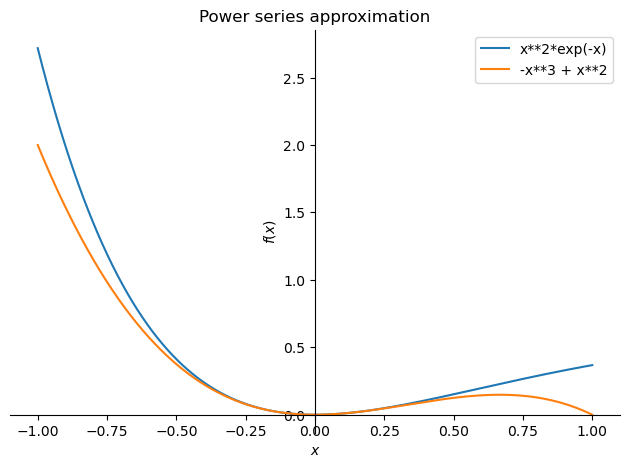

Nonlinear equations¶

With SymPy, we can also solve nonlinear equations or systems of equations algebraically, if possible.

The central function for this is sympy.solve(...). We consider an example in which we compute the stationary points of the function

f(x) = \frac{x}{x^2+1}

(3)

f = x/(x**2+1)
Df = f.diff()
p3 = sy.plot(f,(x,-4,4))  # Plot function

eq = sy.Eq(Df, 0)         # Create equation with lhs DF and rhs 0
sols = sy.solve(eq, x)    # Solve the equation
print("Extrema at", sols) # Print solution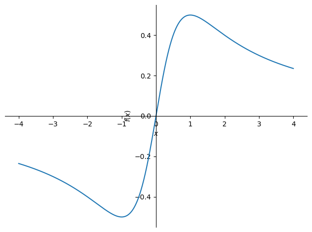

Extrema at [-1, 1]

The stationary points are returned as a list. We can now iterate over them, check which values they are, and evaluate the derivative at these points:

for sol in sols:
    print("Stationary point x =", sol)
    print("Is of type", type(sol))
    print("Satisfies f'(x) =", Df.subs(x, sol))

Stationary point x = -1
Is of type <class 'sympy.core.numbers.NegativeOne'>
Satisfies f'(x) = 0
Stationary point x = 1
Is of type <class 'sympy.core.numbers.One'>
Satisfies f'(x) = 0

Systems of equations can also be solved with sympy.solve. An example:

# Define symbols
x1, x2 = sy.symbols("x1 x2")

# System of equations as a list
equations = [
    sy.Eq(2*x1 + 1*x2, 10),
    sy.Eq(1*x1 - 2*x2, 11) 
]

# Solve the system
sols = sy.solve(equations)
sols

{x1: 31/5, x2: -12/5}

In this case, the result is returned as a dictionary

type(sols)

dict

returned. A dictionary stores key-value pairs: the key is the name of the variable, and the value is its value.

We can iterate over the dictionary entries to output the solutions in an ordered way:

print("The solution of our system of equations is")
for a in sols:
    print(a, "=", sols[a])

The solution of our system of equations is
x1 = 31/5
x2 = -12/5

Alternatively, linear systems of equations can also be solved using sympy.linsolve. Example:

# Define symbols
x1, x2, x3 = sy.symbols('x1, x2, x3')

# Solve linear system of equations
sols = sy.linsolve([2*x1+3*x2-6*x3 - 3, 1*x1-3*x2+3*x3 - 2], (x1, x2, x3))
sols

Since we have 2 equations and 3 unknowns here, we expect infinitely many solutions. linsolve returns these in general in terms of the free variables. With the subs method, we can replace a free variable with a specific value:

for sol in sols:
    print("General solution     :", sol)
    print("Particular solution  :", sol.subs('x3', 0))
    print("Particular solution  :", sol.subs('x3', 2))

General solution     : (x3 + 5/3, 4*x3/3 - 1/9, x3)
Particular solution  : (5/3, -1/9, 0)
Particular solution  : (11/3, 23/9, 2)

Ordinary differential equations¶

Simple differential equations (ODEs) can also be solved with SymPy. First, we need to define the unknown function as a Function and construct the differential equation itself as a symbolic expression. The Derivative method allows us to include derivatives:

x = sy.symbols('x')
y = sy.Function('y')

ode = sy.Derivative(y(x),x,x) + 2*sy.Derivative(y(x),x) - 6*y(x) - sy.exp(3*x)
ode

The differential equation is solved using dsolve:

sol = sy.dsolve(ode, y(x))
print(type(sol))
sol

<class 'sympy.core.relational.Equality'>

The result is an Equality object with a left-hand and a right-hand side. We can extract the right-hand side and use it to create a normal SymPy function:

f = sol.rhs
type(f)

sympy.core.add.Add

The function we just computed depends on the following variables:

f.free_symbols

{C1, C2, x}

Since we did not define any initial conditions, the solution contains two constants C1 and C2. We can replace these with specific values using a dictionary and subs:

constants = {'C1': 1, 'C2': 3}  # Create dictionary
my_f = f.subs(constants)       # Replace constants with values
my_f

Now my_f only depends on x, and we can plot it as usual:

sy.plot(my_f, (x,0,2))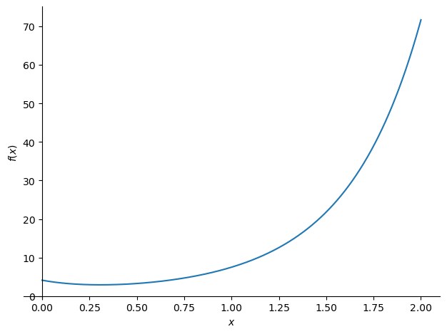

<sympy.plotting.backends.matplotlibbackend.matplotlib.MatplotlibBackend at 0x7cbc67f7e210>

Let us now look at how to solve initial value problems, i.e., differential equations together with corresponding initial conditions. If you call

sy.dsolve?

to view the help text for the dsolve function, you will quickly come across the parameter ics. This expects a dictionary containing the initial or boundary conditions. The following syntax is used:

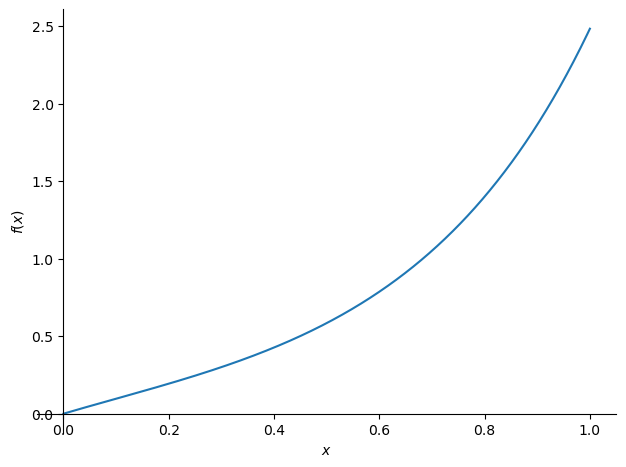
initial_conditions = {y(0)                    : 0, # y(0) = 0
                      y(x).diff(x).subs(x, 0) : 1} # y'(0)= 1

Here, we have specified the initial conditions $y(0)=0$ and $y'(0)=1$ . Calling dsolve now yields:

sol = sy.dsolve(ode, y(x), ics=initial_conditions)
f = sol.rhs
f

Obviously, the solution now only depends on the variable x. This is expected, as the constants of the general solution are determined by the initial conditions.

f from the block above is again a mathematical expression with which we can continue working as usual:

print("f is of type", type(f))
sy.plot(f, (x,0,1))

f is of type <class 'sympy.core.add.Add'>

<sympy.plotting.backends.matplotlibbackend.matplotlib.MatplotlibBackend at 0x7cbc67f7d810>

In the following example, the Riccati differential equation

y'(x) + y(x)^2+\frac{2}{x}\,y(x) = -\frac{2}{x^2}

(4)

is solved. Also of interest is the output of the function sympy.classify_ode(...). SymPy analyzes the differential equation and, depending on the classification, applies an appropriate solution strategy:

ode = sy.Derivative(y(x),x) + y(x)**2 + 2/x*y(x) + 2/(x**2)
sy.classify_ode(ode)

('1st_rational_riccati',
 'Riccati_special_minus2',
 'separable_reduced',
 'lie_group',
 'separable_reduced_Integral')

sol = sy.dsolve(ode, y(x))
sol

f = sol.rhs
my_f = f.subs('C1', 1)
my_f