Mathematical Programming
Preface
In this lecture and the associated exercises, we will get familiar with the programming language Python and its applications in mathematics. The lecture is strongly based on the book Woyand (2021), which can also be downloaded as an e-book from the university library (Link).
What is Python?
Python is a programming language commonly used in web applications, software development, data science, and machine learning. It has also become one of the most important programming languages for mathematical applications, especially in numerical mathematics, data analysis, and scientific computing.
Python is a so-called scripting language, which means that each line of code in the source file is executed sequentially by an interpreter. This simplifies programming because, unlike other programming languages such as C/C++, Fortran, and Java, the code does not need to be compiled into machine code beforehand.
Python is popular among programmers because you can focus more on the problem itself rather than dealing with low-level technical hardware details.
Objectives of the Lecture
In this lecture, we aim to learn the Python programming language and use it to solve mathematical problems. Python becomes particularly powerful through its numerous extension modules. We want to take advantage of these and discuss the following aspects relevant for mathematical applications:
Working with Matrices and Vectors
Beyond typical applications in linear algebra, such as solving linear equation systems, working with matrices and vectors is essential in numerical mathematics. Linear equation systems appear, for example, in the numerical solution of differential equations, in interpolation tasks, and in numerical integration.
Visualization
Graphical representation of solutions is often crucial in mathematics. We will therefore learn how to plot functions and represent datasets effectively in diagrams.
Mathematical Calculations
Python can be used not only as a calculator. There are extension modules that even allow symbolic differentiation and integration, as well as solving nonlinear equations and differential equations symbolically.
Scientific Computing
Many algorithms for a wide range of applications are already implemented in various extension modules, e.g., for numerical optimization, differential equations, nonlinear equations, and integration tasks.
Why Python?
The Python programming language offers several advantages that we can leverage for mathematical applications:
Python is easy to learn, supports common programming paradigms, and is highly readable.
Python is ideal for rapid software prototyping. With just a few lines of code, fairly complex applications can already be written.
There are numerous extensions, called modules, for different applications. In this lecture, we will get to know some of these modules:
NumPy: Working with matrices and vectors
SciPy: Collection of algorithms for scientific computing
SymPy: A computer algebra system for symbolic calculations
Matplotlib: For creating plots and diagrams
Python is portable. Python code runs on all major operating systems (Windows, macOS, Linux).
Python and its modules are freely available. This is an important difference from commercial software like Matlab.
When is Python less suitable?
Python is often less suitable for applications that require high execution speed. Due to dynamic typing and interpreter-based execution, Python is slower in many cases than compiled programming languages. In addition, Python’s flexible data types can lead to relatively high memory usage.
Setup
Before we can implement our first program, we need to set up our computer. We require a Python environment, a suitable editor for writing code, and a way to install external libraries (modules). Below, we present a method that is platform-independent and reliable.
Installing Conda
Conda is a package manager that can be used via the command line. Conda allows you to install packages, including Python itself and external libraries (modules like NumPy, SciPy, and Matplotlib) within an isolated environment.
There are various Conda distributions online. We will use the Miniconda distribution. For all major operating systems, installation files and instructions can be found at https://
For Windows users, it is often recommended to first install the Linux subsystem, see https://
To install Miniconda we open a Linux console and execute the downloaded script with:
cd Downloads
sh Miniconda3-latest-Linux-x86_64.sh
Output:
Welcome to Miniconda3 py313_25.11.1-1

In order to continue the installation process, please review the license
agreement.
Please, press ENTER to continue
During installation, we must accept a license (type yes), optionally provide an alternative installation path, and allow modification of local configuration files (also confirm with yes).
Once installed successfully, open a new terminal and type:
conda listYou should now see a list of all preinstalled packages.
Configuring Conda
In Conda, you can create environments that are largely independent of the rest of the system. In these environments, you can install a Python distribution and additional modules used throughout the lecture.
First, create a new environment named myenv:
conda create --name myenvThis is done only once. To enter the environment later:
conda activate myenvYou will notice that the command prompt changes from:
(base) user@machine:~$to
(myenv) user@machine:~$To test whether Python is installed correctly in this environment:
python3 --versionOutput: Python 3.10.0
We can now start programming in Python. Enter the Python console with:
python3and write our first program, which should print “Hello world!” to the console:
print("Hello world!")Exit the Python console with exit() or CTRL+D. After finishing our work, we can deactivate the Conda environment with:
conda deactivateJupyterLab
Finally, we need a suitable editor for our code. In theory, you could also use Windows Notepad or under Linux gedit, kate, or any text editor. However, it is preferable to use an editor that automatically highlights language-specific keywords (Code Highlighting) and formats the program code neatly (Code Layout).
Popular editors include:
Vim and Emacs (for advanced users)
Python scripts usually have the extension .py (e.g., my_script.py). To run a script from the console, simply type:
python3 my_script.pyThe editor we will use in this lecture is JupyterLab. It works a bit differently than the editors mentioned above. JupyterLab is browser-based and runs in Chrome, Firefox, or another browser.
With JupyterLab, we can not only write plain Python scripts but also interactive notebooks containing code, text, formulas, graphics, and images. More on this later.
We first install the Jupyter notebook directly in our Conda environment:
conda activate myenv
conda install -c conda-forge jupyter
The -c conda-forge option tells Conda to search for the jupyter package also in a public channel called “conda-forge”. Test the installation with:
jupyter --versionOutput: e.g., JupyterLab 6.4.9
Start JupyterLab:
jupyter labA new browser tab should open (possibly in the background).
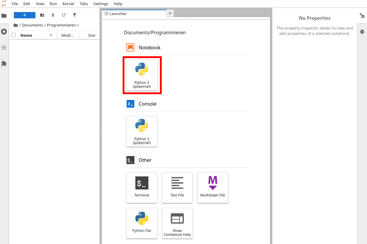
With the Python 3 (ipykernel) button, we can create a new Python notebook and start filling code cells. Execute a code cell with SHIFT+ENTER:
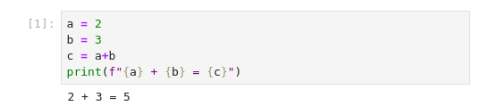
Notebooks are saved with the extension .ipynb. Save changes via File → Save Notebook or CTRL+S.
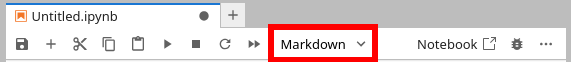
In addition to code cells, Jupyter notebooks contain Markdown cells. To use Markdown cells, switch the dropdown in the toolbar to “Markdown”:
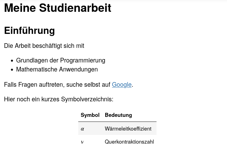
Now we can fill the cell with text and format it nicely. This webpage explains Markdown syntax. We can create headings, embed images and cross-references, create tables and lists, and much more.
Example Markdown code:
# My Thesis

## Introduction

This work deals with:

* Programming Basics
* Mathematical Applications

If you have questions, search on [Google](https://www.google.com).

Here is a short list of symbols:

|Symbol|Meaning|
|:-|:-|
|$\alpha$|Thermal conductivity|
|$\nu$|Poisson's ratio|
Output:
- Woyand, H.-B. (2021). Python für Ingenieure und Naturwissenschaftler. Hanser.