Scientific computing with SciPy - Mathematical Programming

The Python module SciPy is a collection of mathematical algorithms that are primarily used in scientific computing. The module is divided into various submodules. The most important ones are:

scipy.fftpack: Fast Fourier Transform
scipy.integrate: Algorithms for numerical integration and solvers for differential equations
scipy.interpolate: Polynomial and spline interpolation
scipy.linalg: Linear algebra, computations with matrices and vectors
scipy.optimize: Algorithms for solving constrained and unconstrained optimization problems
scipy.signal: Signal processing
scipy.sparse: Storage formats for sparse matrices
scipy.stats: Probability distributions and statistical computations

If necessary, we first need to install SciPy, for example with

conda install -c conda-forge scipy

In the following, we will take a closer look at some of these packages.

Numerical integration with scipy.integrate¶

Numerical integration¶

In the section Computer Algebra with SymPy, we have already learned a method for computing integrals. However, that approach used symbolic computations, meaning it attempted to evaluate an integral exactly. For complicated integrals, a computer algebra system quickly reaches its limits.

An alternative is numerical integration.

The basic idea is to approximate the function by a simpler function, for example by a step function or a piecewise linear interpolation.

import matplotlib.pyplot as plt
import numpy as np

def f(x):
    return np.exp(x)-x
xmin = -2
xmax = 2
x_coarse = np.linspace(xmin, xmax, 8)
x_fine = np.linspace(xmin,xmax,1000)

plt.figure(figsize=(14,4))

plt.subplot(1,2,1)
plt.plot(x_fine, f(x_fine), linewidth=3)
x_tmp = (np.kron(x_coarse, np.array([1.,1.])))[1:-1]
f_tmp = np.kron(0.5*(f(x_coarse[:-1]) + f(x_coarse[1:])), np.array([1.,1.]))
plt.plot(x_tmp, f_tmp, 'r-o', linewidth = 1)
plt.fill_between(x_tmp,f_tmp, alpha=0.5, color='red')
plt.title("Rechtecksregel")

plt.subplot(1,2,2)
plt.plot(x_fine, f(x_fine), linewidth=3)
plt.plot(x_coarse, f(x_coarse), 'r-o', linewidth = 1)
plt.fill_between(x_coarse, f(x_coarse), alpha=0.5, color='red')
plt.title("Trapezregel")

plt.show()

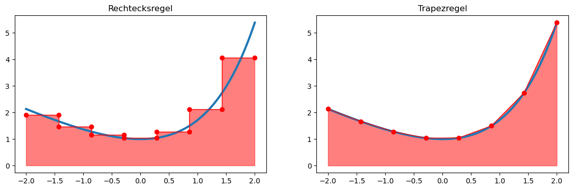
For such functions, the area enclosed by the graph of the function and the $x$ -axis can be computed exactly and easily.

In the composite rectangle rule, the integration domain is first divided into equidistant intervals

I_k = [x_{k-1}, x_{k}],\quad k=1,\ldots,N

(1)

with length

\Delta x = x_{k}-x_{k-1}.

(2)

The step function interpolates the function at the midpoint

\frac12(x_{k-1}+x_{k})

(3)

of the interval.

This leads to the quadrature formula

Q^0(f) = \sum_{k=1}^N f\left(\frac12(x_{k-1} + x_k)\right)\,\Delta x.

(4)

Similarly, for the composite trapezoidal rule, we obtain:

Q^1(f) = \sum_{k=1}^N \frac12\left(f(x_{k-1})+f(x_k)\right)\,\Delta x.

(5)

Computing definite integrals¶

Quadrature formulas, as described above, are implemented in the submodule scipy.integrate. We include this submodule and take a look at the help text of the main function quad (quadrature):

import scipy.integrate as si

si.quad?

Signature:
    si.quad(
        func,
        a,
        b,
        args=(),
        full_output=0,
        epsabs=1.49e-08,
        epsrel=1.49e-08,
        limit=50,
        points=None,
        weight=None,
        wvar=None,
        wopts=None,
        maxp1=50,
        limlst=50,
        complex_func=False,
    )

Docstring:
    Compute a definite integral.

    Integrate func from `a` to `b` (possibly infinite interval) using a
    technique from the Fortran library QUADPACK.

    Parameters
    ----------
    func : {function, scipy.LowLevelCallable}
        A Python function or method to integrate. If `func` takes many
        arguments, it is integrated along the axis corresponding to the
        first argument.

        If the user desires improved integration performance, then `f` may
        be a `scipy.LowLevelCallable` with one of the signatures::

            double func(double x)
            double func(double x, void *user_data)
            double func(int n, double *xx)
            double func(int n, double *xx, void *user_data)

        The ``user_data`` is the data contained in the `scipy.LowLevelCallable`.
        In the call forms with ``xx``,  ``n`` is the length of the ``xx``
        array which contains ``xx[0] == x`` and the rest of the items are
        numbers contained in the ``args`` argument of quad.

        In addition, certain ctypes call signatures are supported for
        backward compatibility, but those should not be used in new code.
    a : float
        Lower limit of integration (use -numpy.inf for -infinity).
    b : float
        Upper limit of integration (use numpy.inf for +infinity).
    args : tuple, optional
        Extra arguments to pass to `func`.
    full_output : int, optional
        Non-zero to return a dictionary of integration information.
        If non-zero, warning messages are also suppressed and the
        message is appended to the output tuple.
    complex_func : bool, optional
        Indicate if the function's (`func`) return type is real
        (``complex_func=False``: default) or complex (``complex_func=True``).
        In both cases, the function's argument is real.
        If full_output is also non-zero, the `infodict`, `message`, and
        `explain` for the real and complex components are returned in
        a dictionary with keys "real output" and "imag output".

    Returns
    -------
    y : float
        The integral of func from `a` to `b`.
    abserr : float
        An estimate of the absolute error in the result.
    infodict : dict
        A dictionary containing additional information.
    message
        A convergence message.
    explain
        Appended only with 'cos' or 'sin' weighting and infinite
        integration limits, it contains an explanation of the codes in
        infodict['ierlst']

As function parameters, scipy.integrate.quad requires a reference to the function to be integrated as well as the integration bounds.

The return value is a tuple containing

the approximated value of the integral
an estimate of the integration error.

A simple example:

import math

def f(x):
    return math.exp(x) - x

res, err = si.quad(f, -2., 2.)

print("Integral           :", res)
print("Estimated error    :", err)

Integral           : 7.253720815694037
Estimated error    : 8.053247863786291e-14

Multiple integrals¶

Double and triple integrals (i.e., surface and volume integrals) can also be computed with scipy.integrate. Suppose we want to integrate a scalar field $f\colon \mathbb{R}^2\to \mathbb{R}$ over a region

D=\{(x,y)\in \mathbb R^2\colon x\in [a,b],\; y\in [g(x), h(x)]\}

(6)

Thus, the integration is not limited to rectangular domains ( $g, h\equiv \text{const}$ ); the integration bounds of the inner variable (here $y$ ) may also depend on the outer variable (here $x$ ).

In the following example, the function

f(x,y) = x^2\,e^y

(7)

is integrated over the triangular region

\{(x,y)\colon x\in [0,1],\; y\in[0,1-x]\}

(8)

def f(y, x):
    return x**2 * math.exp(y)

def g(x):
    return 0

def h(x):
    return 1 - x

res, err = si.dblquad(f, 0, 1, g, h)
print("Integral           :", res)
print("Estimated error    :", err)

Integral           : 0.10323032358475713
Estimated error    : 1.9673235155680954e-15

In an analogous way, a triple integral (volume integral) can also be computed using the function scipy.integrate.triquad.

Optimization problems with scipy.optimize¶

Preliminary considerations¶

With the submodule scipy.optimize, we can solve optimization problems of the form

\begin{aligned} f(x) &\to \min!\quad &&\text{over}\quad x\in \mathbb{R}^n &&\text{(objective function)}\\ g_i(x) &\le 0 &&\text{for}\ i=1,\ldots,m &&\text{(inequality constraints)}\\ h_j(x) &= 0 &&\text{for}\ j=1,\ldots,p &&\text{(equality constraints)}\\ a_k \le x_k &\le b_k &&\text{for}\ k=1,\ldots,n&&\text{(box constraints)} \end{aligned}

(9)

solve.

Note that box constraints are also inequality constraints. However, there are optimization methods that are specifically tailored to problems with box constraints and can work particularly efficiently by exploiting this structure.

If no constraints are given, this is referred to as an unconstrained optimization problem.

Let us first look at how we can solve such optimization problems. To do this, we import the submodule and read the help text of the main function minimize:

from scipy import optimize

optimize.minimize?

Signature:
optimize.minimize(
    fun,
    x0,
    args=(),
    method=None,
    jac=None,
    hess=None,
    hessp=None,
    bounds=None,
    constraints=(),
    tol=None,
    callback=None,
    options=None,
)
Docstring:
Minimization of scalar function of one or more variables.

Parameters
----------
fun : callable
    The objective function to be minimized::

        fun(x, *args) -> float

    where ``x`` is a 1-D array with shape (n,) and ``args``
    is a tuple of the fixed parameters needed to completely
    specify the function.
x0 : ndarray, shape (n,)
    Initial guess. Array of real elements of size (n,),
    where ``n`` is the number of independent variables.
args : tuple, optional
    Extra arguments passed to the objective function and its
    derivatives (`fun`, `jac` and `hess` functions).
method : str or callable, optional
    Type of solver.
jac : {callable,  '2-point', '3-point', 'cs', bool}, optional
    Method for computing the gradient vector. Only for CG, BFGS,
    Newton-CG, L-BFGS-B, TNC, SLSQP, dogleg, trust-ncg, trust-krylov,
    trust-exact and trust-constr.
    If it is a callable, it should be a function that returns the gradient
    vector::

        jac(x, *args) -> array_like, shape (n,)

    where ``x`` is an array with shape (n,) and ``args`` is a tuple with
    the fixed parameters.
hess : {callable, '2-point', '3-point', 'cs', HessianUpdateStrategy}, optional
    Method for computing the Hessian matrix. Only for Newton-CG, dogleg,
    trust-ncg, trust-krylov, trust-exact and trust-constr.
hessp : callable, optional
    Hessian of objective function times an arbitrary vector p. Only for
    Newton-CG, trust-ncg, trust-krylov, trust-constr.
bounds : sequence or `Bounds`, optional
    Bounds on variables for Nelder-Mead, L-BFGS-B, TNC, SLSQP, Powell,
    trust-constr, COBYLA, and COBYQA methods.
constraints : {Constraint, dict} or List of {Constraint, dict}, optional
    Constraints definition. Only for COBYLA, COBYQA, SLSQP and trust-constr.
tol : float, optional
    Tolerance for termination.
options : dict, optional
    A dictionary of solver options.
callback : callable, optional
    A callable called after each iteration.

Returns
-------
res : OptimizeResult
    The optimization result represented as a ``OptimizeResult`` object.
    Important attributes are: ``x`` the solution array, ``success`` a
    Boolean flag indicating if the optimizer exited successfully and
    ``message`` which describes the cause of the termination. See
    `OptimizeResult` for a description of other attributes.

As function parameters, minimize requires at least a reference to the objective function as well as an initial value x0. The objective function may have the form

def f(x):
    return x**2

A simple example:

import numpy as np

def f(x):
    return np.power(x, 3) - np.power(x, 2) - 15*x

x0 = 0
sol = optimize.minimize(f, x0)
sol

  message: Optimization terminated successfully.
  success: True
   status: 0
      fun: -28.18423549805634
        x: [ 2.594e+00]
      nit: 4
      jac: [-1.669e-06]
 hess_inv: [[ 7.378e-02]]
     nfev: 16
     njev: 8

The return value is a structure of type OptimizeResult. In addition to the found solution sol.x, this object also contains further useful information about the optimization process. For example, we can see how many iterations were required and how often the objective function or its derivatives were evaluated.

Let us now plot the function and check whether the found minimum is plausible:

import matplotlib.pyplot as plt

x = np.linspace(-2,5,1000)
y = f(x)

plt.plot(x,y)
    
plt.scatter(float(sol.x[0]), sol.fun, marker='o', color='red')
plt.legend(['Function', 'Minimizer'])
plt.show()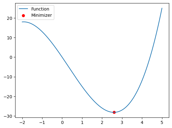

Unconstrained optimization problems¶

What actually happens inside the minimize function? Depending on the problem, a numerical method for solving the optimization problem is selected and applied.

Most numerical methods for unconstrained optimization problems generate a sequence of iterates

x_{n+1} = x_n + s_n\,d_n,\quad n=0,1,\ldots,

(10)

where $x_n$ is the current iterate, $d_n$ is a suitable search direction, typically a descent direction, and $s_n$ is a step size. This procedure is repeated until a stopping criterion is satisfied, for example

\|\nabla f(x_n)\| \le \varepsilon .

(11)

The simplest of these methods is the so-called gradient method, where the search direction is given by

d_n = -\nabla f(x_n).

(12)

A suitable step size can be obtained using a so-called line-search method, for example with Armijo backtracking.

Since we did not provide the gradient to minimize, it is internally replaced by a finite difference approximation. However, the algorithm works more efficiently if we provide the gradient explicitly:

def Df(x):
    return 3*np.power(x, 2) - 2*x - 15

sol = optimize.minimize(f, x0, jac=Df)
sol

  message: Optimization terminated successfully.
  success: True
   status: 0
      fun: -28.184235498056328
        x: [ 2.594e+00]
      nit: 4
      jac: [-1.952e-06]
 hess_inv: [[ 7.378e-02]]
     nfev: 8
     njev: 8

Compared to our first attempt, we saved some function evaluations here, namely those required to approximate the gradient.

However, it is still unclear which optimization algorithm is actually used. In many cases, a so-called (quasi-)Newton method is applied. In this approach, the search direction is determined using the Hessian matrix:

d_n = -\nabla^2 f(x_n)^{-1} \nabla f(x_n)

(13)

This requires solving a linear system involving the Hessian matrix $\nabla^2 f(x_n)$ .

If we are able to compute this Hessian explicitly, we can also pass it to the minimize function:

def DDf(x):
    return 6*x - 2

sol = optimize.minimize(f, x0, jac=Df, hess=DDf, method="Newton-CG")
sol

 message: Optimization terminated successfully.
 success: True
  status: 0
     fun: -28.184235498056466
       x: [ 2.594e+00]
     nit: 5
     jac: [ 1.017e-04]
    nfev: 7
    njev: 7
    nhev: 5

Here, we have also explicitly specified that minimize should use a Newton method (Newton-CG).

Optimization problems with constraints¶

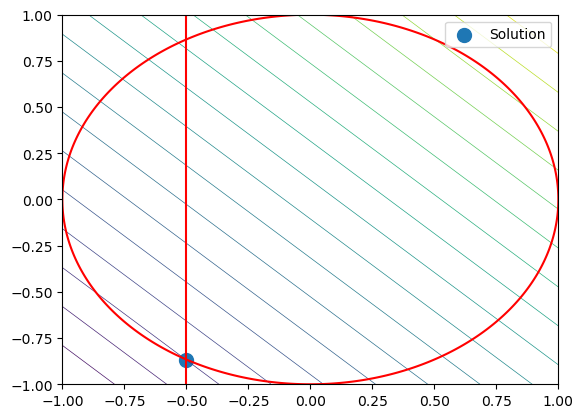
Let us consider a second optimization problem with objective function

f(x,y) = x+y\to \min!

(14)

and one equality and one inequality constraint

\begin{aligned} g(x,y) &= x+0.5 \ge 0\\ h(x,y) &= x^2+y^2 -1 = 0. \end{aligned}

(15)

The equality constraint describes the unit circle, while the inequality constraint further restricts the feasible region by the condition (x \ge -0.5).

First, we define the objective function, its gradient, and the constraints:

# Objective function
def f(x):
    return x[0] + x[1]

# Gradient of the objective function
def Df(x):
    return np.array([1., 1.])
    
# Equality constraint
def h(x):
    return x[0]**2 + x[1]**2 - 1

# Jacobian of the equality constraint
def Dh(x):
    return np.array([2*x[0], 2*x[1]])

constraints = [{'type': 'eq', 'fun': h, 'jac': Dh}]
bounds = [(-0.5, None), (None, None)]

x0 = np.array([-0.2, 0.])

sol = optimize.minimize(f, x0, jac=Df, bounds=bounds, constraints=constraints)
sol

     message: Optimization terminated successfully
     success: True
      status: 0
         fun: -1.3660254050073637
           x: [-5.000e-01 -8.660e-01]
         nit: 5
         jac: [ 1.000e+00  1.000e+00]
        nfev: 5
        njev: 5
 multipliers: [-5.774e-01]

To visualize the problem, we plot the objective function, the equality constraint, and the box constraint:

x = y = np.linspace(-1,1,1000)
X,Y = np.meshgrid(x,y)

Z = f([X,Y])
H = h([X,Y])

# Plot objective function
plt.contour(X,Y,Z, linewidths=.5, levels=np.linspace(np.min(Z), np.max(Z), 20))

# Plot constraint h(x,y)=0
plt.contour(X,Y,H, levels=[0.], colors="red")

# Plot box constraint
plt.plot([-0.5, -0.5], [-1., 1.], 'r-')

# Plot solution
plt.scatter(sol.x[0], sol.x[1], marker="o", s=100, label="Solution")

plt.legend()
plt.show()